How To Unhide Or Hide Rows In Google Sheets – 4 Tested Ways

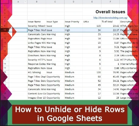
Hidden rows in Google sheets can be very frustrating for the ones who don’t know how to unhide them. It’s a simple process to unhide them. Conversely, if you are working on big data on google sheets or sharing a spreadsheet with someone but you don’t allow them to see the rows you’ve already hidden. In this guide, I’ll take you through How To Unhide or Hide Rows in Google Sheets. 

I checked and found 4 tested ways to unhide the hidden rows. And several ways to hide rows or columns in Google Sheets. So, without beating about the bush let’s check if the Rows are hidden or not

Note: You can apply the same trick to hide or unhide columns in Google Sheets.

Check If The rows are Hidden or Not.

Most of the time it happens while searching data on spreadsheets you are not able to find. It could be you mistakenly hide some rows or you delete the rows and now you are more worried about the data.

Primarily, Make sure you hide the rows or they are deleted accidentally. In other cases, you send your file to your boss and the boss is not able to find the important data. If the rows are hidden mistakenly check the very first step below.

Go to the top left corner of the Google Sheet Page, Click on the gray rectangle and your entire page will be selected

Now, right-click on the page and check the “unhide rows” option in the menu if you the option it means the rows are hidden. If you don’t see that option it means, there are no hidden rows on your google sheet.

Anyhow, If you find “unhide rows” and click on it will not do anything. It merely shows the existence of the hidden rows. To unhide rows we have gathered all the possible ways below.

4 Tested Methods To Unhide Rows in Google Sheets

1. First: Use Arrows for unhiding the rows
2. Second: Unhide rows by selection
3. Third: Keyboard Shortcut CTRL + SHIFT + 9
4. Forth: Use Filter to Unhide Rows

First: Use Arrows for unhiding the rows

First of all, Go to the spreadsheet that has hidden rows and you want to unhide them.

Click on the arrow – in the rows line you will see many up and down arrows. Click any of them to check unhidden rows. 

If you don’t find the rows use Keyboard Shortcut to unhide.

Second: Keyboard Shortcut CTRL + SHIFT + 9

Open the sheet which has hidden rows. Select all the data from the row heading to the bottom with a cursor or press CTRL + A from your keyboard.

Once all the data is selected (highlighted). Use Keyboard shortcut for ease. Press CTRL + SHIFT + 9. It will unhide all the rows on the google sheet.

Third: Unhide rows by selection

Similar to the above method. Go to the sheet which has hidden rows, open it, and select all rows including all the data with the help of a cursor (mouse).

Now, Once all the data is selected. Right-Click anywhere on the sheet and you will “unhide rows” option. Click and all done.

You would be able to see all the hidden data.

Forth: Use Filter to Unhide Rows

The last but not least method. Some data may not appear in the sheet due to filters. Filters can sometimes hide rows. A sheet does not display any indication that hidden data is hidden, such as arrows in a row heading or the option to unhide rows. If there are no arrows or missing row numbers in row headings, you can verify that hidden rows exist.

For Example, If you see 5,7,9 rows are missing without any arrows it shows that these rows are hidden by filter option. Simply turn off the filter option and all the rows will be visible.

Click on the Remove Filter icon to turn off all the filters already applied on the sheet. Once you click you will see all the unfiltered rows immediately.

Another way to disable filters. Just go to the Data Tab at the top of the sheet. Click on Remove filter option. This way all the filters may disappear from your sheet and you would be able to see all your data.

Note: By using the same methods you can check how to unhide columns in Google sheets.

These are the four methods through which you can check your hidden data. Now, If you also want to know How To Hide Rows in Google Sheets. You better continue reading till the end.

How To Hide Rows in Google Sheets

For hiding a single row, right-click on the row number on the left side of the sheet and select the row – Right-click and hide row.

If you want to hide multiple rows at once. Click on the first row and drag till the row you want to hide or use keyboard Shift + Down keys for dragging.

Once you select the range of the rows you want to hide. Right-click and click hide-rows or use keyboard shortcut SHIFT + ALT + 9. Your selected rows will be hidden this way.

By the same token, use the above methods to Hide columns in google sheets.

Final words

After reading the post I hope now you are aware of the methods on how to unhide rows in Google sheets by using keyboard shortcuts or selecting the ranges. On the contrary, how to hide rows in Google Sheets. If you know any other way to hide or unhide rows and columns. Please share with us in the comment section. Thank you for reading and staying with Technob.